|
|
The previous chapter covered general issues in costing. This chapter looks at some practical aspects of costing, specifically:
All these are practical extensions of the concepts developed in Chapter 11.
As pointed out in the previous chapter, costing is generally a means to an end. One of the ends is to measure performance. We may want to know whether a government entity is operating efficiently; is it producing a given output at least possible cost, or, for a given cost of input, is it maximizing its useful output?
In competitive markets financial ratios (such as return on equity, or return on funds
employed) will often give some indicator of a firm's efficiency. In the public sector such
measures, even when available in GBEs, are rarely useful. Impressive financial results may
result from exploiting a monopoly situation (covered in Chapter 15). They may result from
access to finance at low rates of interest or exemption from certain taxes. On the other
hand, government entities may be burdened with specific community service obligations, may
have expensive accountability requirements, and they may have conditions of employment
which render labor costs higher than in the private sector. In the absence of useful
"bottom line" indicators, many partial indicators may be used, including productivity
indicators, to see how efficiently government entities are using their capital and labor
resources.
Labor/Capital Intensities
Government activities can be classified into a capital intensive group
and a labor intensive group. Capital intensive government
industries include electricity generation and distribution, communications, and water
supply. Telstra, for example, in 1999-2000 had assets per employee of $600 000 and
turnover per employee of $400 000. It is no coincidence that many capital intensive
industries are in the public sector; capital intensity is one of the aspects of natural
monopoly, which is often leads to public ownership. The concept of natural monopoly is
covered in Chapters 15 and 16. On the other hand many government activities, including
education, health care, law and public safety, and public administration, are relatively
labor intensive.
Measuring Productivity
Productivity is a loosely defined, and easily manipulable term, referring generally to measures of output divided by input. A single measure of productivity has little meaning in itself; generally measures of productivity are used for comparison over time or between enterprises.
The main measures of productivity are:
labor productivity - output per unit of labor input. Both numerator and denominator need defining. Output may be in dollar amounts, such as total turnover, or value-added. It may be expressed in terms of physical units. Input may the number of employees, or the number of hours worked. There is a political art in choosing the measure which advances a particular argument. If we want to show Telstra has low productivity, we point out it has only 88 lines per employee, compared with 196 for US telecom companies. Conversely, if we want to show the efficiency of Qantas, we point out that in terms of tonne kilometers per employee, it was 6 percent more efficient than United and 36 percent more efficient than British Airways.(1) The 1998-99 waterfront dispute gave rise to many countervailing measures about labor productivity, with claims that the number of containers moved per employee in Australian ports was only half the number moved in large European ports.(2) The research on which this finding was based was heavily qualified - European ports had larger cranes, better scale economies, and the measure of labor productivity was based on person years, not hours worked. These nuances were ignored in the heat of the political slanging match.
One standard method of measuring labor productivity is to use the national accounts basis of measuring value-added, in constant prices, divided by hours worked. This has a certain appeal of objectivity, but being measured in currency terms it becomes removed from physical productivity; a real price rise arising from extraneous factors or exploitation of a monopoly position in a market can contribute to an apparent rise in productivity.
capital productivity - output per unit of capital input. Sometimes it is measured by reference to capital stock, sometimes by reference to capital consumption. Rarely can we use simple measures for input, however, other than to get some crude measures such as tonnes of freight per wharf, etc. In the waterfront dispute there were many measures of capital productivity in the form of containers per crane per hour - around 18 in Australia's case compared with around 25-30 in European ports. Again, such measures are fraught with difficulties in interpretation - there are many difficult types of cranes (some can lift two containers at a time) and many different types of container.
A commonly used estimate of capital productivity is to find some measure of value-added divided by some estimate of the value of capital stock. These estimates are subject to all the problems of asset valuation mentioned in Chapter 4.
Movements in capital and labor productivity tend to offset each other in the short term at least. Investment in labor saving equipment will generally increase labor productivity while decreasing capital productivity. (An exception occurs when the price of capital equipment tumbles, as has happened in some communication technologies.) There is therefore a quest for a single measure of productivity, which combines labor and capital.
total factor productivity (TFP) - output (or change in output) divided by some weighted index of labor and capital input. Because of this weighting it will always be somewhere between the measures of labor and capital productivity.
There is also the potential for measures of resource productivity, such as output divided by some intermediate mineral or other resource based input - tonnes of steel per tonnes of iron ore, production of carbohydrate per liter of water etc. These are becoming more important in a world conscious of limits in natural resources.
Exercise
A government enterprise has had the following performance (figures in current prices). It has invested heavily, and has reduced staff in a productivity agreement. What was its growth in labor, capital and total factor productivity? To obtain TFP you can weight labor by 0.6 and capital by 0.4. (Over the period the CPI, which can be used to deflate current prices, moved from 120.2 to 124.7.)
| 1998 | 2000 | |
| Output ($ million) | 1000 | 1110 |
| Inputs (non-labor) ($ million) | 400 | 410 |
| Employees | 2000 | 1900 |
| Annual hours per employee | 1700 | 1695 |
| Capital stock ($ million) | 2000 | 2300 |
The spreadsheet for this exercise is at ch12ex01.xls. The exercise is designed mainly to show a typical
derivation of total factor productivity, and the limits of single measures, be they labor
or capital. Impressive developments in labor productivity are often simply the result of
investment in capital to replace labor, or, sometimes, contracting out, which reduces the
"in house" workforce, which is the basis for labor productivity measures.
Productivity Comparisons Between Enterprises
It is also possible to get comparisons in productivity
between different entities, but such measures should be treated with extreme caution.
Differences can come about because of differences in geography, climate, differences in
related industries. For example, an urban rail system is only part of the public transport
system, which in turn is only part of the urban transport system. Different cities have
different layouts, landforms, population densities, and ages. Comparative performance
data, even when collected on similar bases, can be almost meaningless.
Exercise
As an example ch12ex02.xls shows performance data for Australian urban bus systems in 1993. (There is not such a set of data available for later years, as privatized companies are subject to much less openness in their reporting.) You can use this spreadsheets to derive various comparative performance indicators. (There are some suggested indicators in the remplate, but you will probably have others.) Use your knowledge of local geography, population and other infrastructure to help in your interpretation.
Labor Intensive Industries - Measuring Labor Costs
By contrast with GBEs, for many core government activities, like education and health care, it is very hard to measure productivity. Some simple output/labor input productivity measures are available, but these are more akin to performance indicators rather than to total productivity measures. By convention productivity gains in such industries are assumed in national accounts to be zero, although some measures are being developed.
This is not to say productivity gains cannot be achieved in such industries. It's just that they're hard to measure. A useful starting point in such industries is to ensure there is adequate awareness of labor costs. Managers in public sector agencies often consider labor to be a sunk cost - they will call a two hour meeting of ten staff over a trivial matter, for example, without considering the cost of such a gathering.
Exercise
Develop a model to come up with an acceptable figure (for charge-out purposes) for the hourly cost of an employee with an annual pay of $50 000. Make allowance for the following costs:
| Superannuation | 12% |
| Workers' compensation | 3% |
| Leave loading | 2% |
| Average expenditure on rent, telephone, stationery | $30 000 |
| Corporate support per head | $5 000 |
| Four weeks leave a year Six public holidays a year Seven days sick leave and furlough |
|
| Basic working day | 7.3 hours |
| Housekeeping (filing etc) | 30 mins a day |
| Keeping abreast (reading circulars etc) | 15 mins a day |
| Personal time | 18 mins a day |
A form of the model is in the spreadsheet at ch12ex03.xls. Your model will be richer if you substitute figures based on your experience. Once you have a figure, consider the cost, say, of a two hour meeting involving ten staff.
There are many arguments about what factors to use in costing labor. Should average sick leave figures be used, even among staff who take little sick leave? Should all management overheads be charged back to the program staff - after all it's not their choice to maintain an expensive security system, or to hire cleaners who come in once a day? Should average or marginal costs be used - what if we can expand our operations without expanding managerial overheads?
Sometimes central government agencies publish and apply service-wide factors for costing labor. For example, in a misinterpretation of the Commonwealth Department of Finance and Administration guidelines, many public sector managers simply load a 154 percent absorption factor on top of salary costs to find total cost. (The handbook on which this factor is based is out of date, and the figure is used as an example only, but it is still used as an authoritative source by many managers, and by those who have an ideological bias towards measures which show in-house" operations to be expensive.(3)
In general, we should resort to such published factors
(called absorption factors) only if we do not have the data to
generate the information for our own agency. A stand-alone outfit, with its own management
support, paying its own rent, will have enough costing information to generate its own
cost data. Use of published allocation factors is a quick and dirty way of generating cost
data, and should not be used for major decision-making.
In the last chapter we introduced cost and volume relationships. A simple exercise will illustrate the topic here.
Exercise
An electricity authority has the following cost structure:
| ($ million pa) | |
| Fixed costs | |
| Labor | 600 |
| Depreciation | 150 |
| Other operating costs | 100 |
| Return on capital | 6 percent |
| Variable costs | |
| Machine wear | $0.004 per KwH |
| Coal | see below |
Its assets are valued at $5 000 million and its generating capacity, using modern equipment, is 35 000 million KwH per year. (It has some older equipment on standby, but hasn't needed to swing it into action.)
The authority has its own coal reserves. Each tonne of coal can produce 1600 million KwH of electricity. The authority has never exported the coal, but if it did it could get an export value of $60 a tonne at the nearest seaport. Freight to the seaport would be $10 a tonne.
Develop two cost models of this enterprise - one a total cost model, the other a variable cost model.
The first step is to separate the fixed and variable cost elements. The fixed cost elements are fairly straightforward. (We should remember to include return on assets as a fixed cost.)
The coal should be valued at its opportunity value, which is its export value. This comes to $50 a tonne, or $0.03125 (= 50/1600) per KwH generated, or $0.03125 million per million KwH. The other variable cost element ($0.00400 per KwH) relates to machine wear - the more we use the machinery the more we will need to spend on maintenance, parts, and lubricants.
We can thus develop a model, incorporating these input
variables. We should give ourselves the capacity to vary these inputs. The model is at ch12ex04.xls.
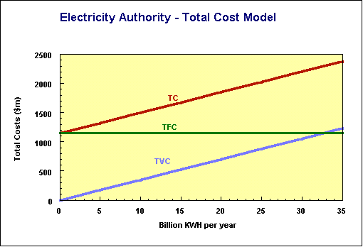
Total and Unit Cost Models
The graphs below are models of the power utility, just as the spreadsheet from which they were derived is a model. The key points on the total cost graph are:
Fixed costs - TFC which is a straight line of $1 150 million a year, regardless of output;
Variable costs - TVC which in our example is a straight line, sloping upwards. In other words the variation is linear; the rise in TVC as we go from 10 000 to 20 000 million KwH is the same as the rise as we go from 20 000 to 30 000 million KwH. In other cases the relationship may be non-linear;
Total costs - TC which is a straight line in this case, moving upwards from the FC line.
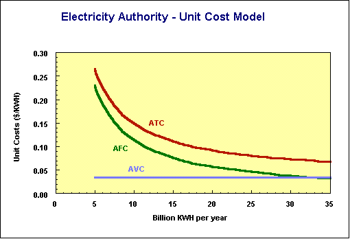
The second graph shows the same information as unit costs.
Exercise
Looking at the power generating model, consider the following two scenarios, both based on the authority generating and selling 30 000 million KwH of electricity a year (at which point its average cost per KwH is $0.74).
1.Due to an upturn in the Japanese economy, the export price of coal rises to $80 a tonne. What does our model now show for unit total cost (ATC)? Should the price rise accordingly, and, if so, how should it be explained to consumers?
2.The Government is considering electrifying the main trunk railroads, which would require an extra 1 000 million KwH a year of electricity. It knows the electricity authority's cost structure. What price should it reasonably expect to pay - a marginal cost of $0.35, or an average cost of $0.74 per KwH?
Break-even analysis is a simple but powerful analytical modelling tool. Imagine that this power utility sells its output for 8 cents a KwH. We can then add a revenue line to the total cost model developed above. The model, modified with a break-even line, is at ch12ex05.xls.
Where the revenue and cost lines cross (25 555 MKwH) is called the break even point. At higher levels of throughput the authority makes a profit, at lower levels it makes a loss.
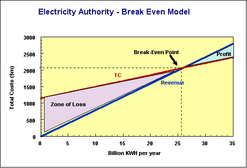
Another concept associated with break even analysis is contribution,
which is the difference between unit variable cost and unit revenue. It is called contribution
as a shorthand way of saying "contribution to fixed costs and
profit". In this case the contribution is 4.5 cents per unit (8.0 revenue less 3.5
variable cost). That contribution has to absorb fixed costs of $1150 million. Therefore
the break even point is 25 555 MKwH (1150/0.045).
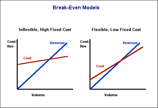
Break Even Models and Firms' Behavior
Look at the two models below. On the left is a firm with almost entirely fixed costs; on the right a firm with almost entirely variable costs.
Note that firms with high fixed cost have high
contribution. They either make high profits or high losses. There are large incentives to
increase sales, through promotion or securing access to privileged markets. There will be
incentives to cut price to gain market share, just as long as there is a positive
contribution. Industries with such firms are prone to price wars, heavy promotional
activity, and general market instability. They are also prone to monopolization, a point
to which we return in Chapter 15 when we look at pricing. They include private sector
industries such as airlines, pharmaceuticals, and petrochemicals, and many GBEs which are
in the public sector because they are natural monopolies, a point to which we return in
Chapter 14..
We have already discussed the basic issues in overhead
allocation in Chapter 11. The two following exercises illustrate some practical points.
Exercise
Throughout Australia now there is pressure on water and sewerage authorities to separate their costs for water and sewerage.(4) Conceptually that is reasonable, but in practice it is difficult. The exercise below simulates a small water and sewerage authority, as may be serving a coastal community of, say, 20 000 to 30 000. Its total annual costs are $2 million, of which $830 000 cannot be traced directly to either water or sewerage.
| Water | Sewerage | Joint (non-traceable) | Total | |
| Basic Operating Figures | ||||
| Assets $m | 4 000 000 | 2 000 000 | 1 000 000 | 7 000 000 |
| Megaliters handled | 2 000 | 160 | 2 160 | |
| Employees | 5 | 8 | 15 | 28 |
| Costs $pa | ||||
| Return on assets (7%) | 280 000 | 140 000 | 70 000 | 490 000 |
| Labor costs | 170 000 | 225 000 | 650 000 | 1 045 000 |
| Materials | 30 000 | 20 000 | 5 000 | 55 000 |
| Depreciation (3%) | 120 000 | 60 000 | 30 000 | 210 000 |
| Other | 55 000 | 70 000 | 75 000 | 200 000 |
| Total | 655 000 | 515 000 | 830 000 | 2 000 000 |
Knowing that costing is often a precursor to charging,
various parties in the community have been arguing for different bases for costing:
market gardeners argue that the authority exists basically to supply sewerage to the community. People could supply their own water from pumps, wells and rainwater tanks, but sewerage is essential for environmental reasons. They argue that water supply is only a marginal operation for the authority, and should be costed accordingly. On this basis they arrive at a cost of $328 a megaliter for water and a cost of $8 406 per megaliter of sewerage handled;
tourist accommodation owners argue that the most rational way to charge is on the objective measure of the volume of material handled. On this basis they arrive at a cost of $743 a megaliter for water and a cost of $3 219 per megaliter of sewerage handled.
Which argument has more validity? Are there more valid ways of costing the two products?
A spreadsheet is at ch12ex06.xls. The extreme treatments load all joint costs into one product, leaving the other product to cover only traceable costs. This is close to costing one product at its avoidable costs only, while costing the other product at its stand alone costs.
There can be more than one basis of allocation - for
example allocating non-traceable labor costs by traceable employment, non-traceable
material costs by traceable material, etc. Arguments over cost allocation are very common.
While some methods have more logical appeal than others, there is no one correct way - by
definition because these costs are untraceable.
Exercise
A government education authority has decided to let the private sector compete to provide counselling services. Its own counselling services will be maintained, but they must break even and determine an appropriate pricing structure.
The typical government counselling center provides two types of service for students:
(1) Twenty minute interviews with trained counsellors, whose direct labor costs (including superannuation, leave and workers' compensation insurance) are $24.00 an hour (2000 interviews a year);
(2)Twenty minute interviews with qualified psychologists, whose direct labor costs are $42.00 an hour (1500 interviews a year).
All counsellors, regardless of status, have the same design of offices and access to other facilities in the counselling centers. (They move around counselling centers as the need arises.) The annual overhead cost for a counselling center is:
| Rent | $40 000 |
| Utilities & phone | $20 000 |
| Receptionist | $35 000 |
| Other | $45 000 |
| Total | $140 000 |
The Department of Budget, referring to its costing handbook, recommends that the government counselling center charge fees on a cost recovery basis of $38.27 per counsellor interview and $66.97 per psychologist interview. Its calculations are below.
| Counsellor | Psychologist | Total | |
| Interviews | 2 000 | 1 500 | 3 500 |
| Time per interview | 0.33 | 0.33 | |
| Direct cost per hour | $24.00 | $42.00 | |
| Direct cost per interview | $8.00 | $14.00 | |
| Annual direct costs | $16 000 | $21 000 | $37 000 |
| Percentage of annual direct costs | 43.24% | 56.76% | 100.00% |
| Overheads | $140 000 | ||
| Allocated proportional to direct costs | $60 541 | $79 459 | |
| Overheads per interview | $30.27 | $52.97 | |
| Total cost per interview | $38.27 | $66.97 |
What would be likely to happen if the counselling centers implemented the recommended fees? What fees would you recommend? The method in the above table is reasonably transparent; a spreadsheet is at ch12ex07.xls.
This exercise is a warning about automatically linking cost estimates to pricing. As we will point out in Chapters 14 and 15, costing and pricing are different exercises, serving different purposes.
Specific References
1. EPAC Council Paper #14 The Size and Efficiency of the Public Sector (EPAC 1990)
2. Bureau on Industry Economics Waterfront 1995, International Benchmarking (BIE 1995)
3. Commonwealth Department of Finance Guidelines for Costing of Government Activities (AGPS July 1991)
4. Industry Commission Water Resources and Waste Water Disposal Draft Report (IC March 1992)