|
|
Spreadsheets are powerful management tools. Next to word processing, they are probably the most widely used application on desktop computers.
There are many different spreadsheets - Lotus, Excel, Multiplan, Quattro Pro etc - but at a basic level they all obey the same rules of structure.
Imagine you are catering for drinks for 20 people, and will be supplying beer, wine, orange juice, cheese, crackers and chips. If you're well organized you'll take out a sheet of paper, rule it into columns and rows, and plan along the following lines:
| No guests | 20 | |||||||
| Item | Cons per head | Total need | Price per pack | Pack size | No packs | Total price | ||
| Beer | 500 | ml | 10 000 | $5.10 | 750 | ml | 14 | $71.40 |
| Wine | 120 | ml | 2 400 | $12.68 | 750 | ml | 4 | $50.72 |
| OJ | 200 | ml | 4 000 | $4.00 | 2000 | ml | 2 | $8.00 |
| Cheese | 120 | gm | 2 400 | $7.80 | 1000 | gm | 3 | $23.40 |
| Crackers | 100 | gm | 2 000 | $2.25 | 300 | gm | 7 | $22.75 |
| Chips | 150 | gm | 3 000 | $3.20 | 375 | gm | 8 | $25.60 |
| Total Outlay | $201.87 | |||||||
| Per head | $10.09 | |||||||
That's fine, until someone tells you there will be 27 guests. You work it out again. And your mate Shirley can get beer for $4.80 a bottle, and you might need something upmarket in the cheese line - $11.70 a kilo, and these are big beer drinkers, allow 700 ml a head, that all costs too much, can we get it down below $11.00 a head ...
That's where spreadsheets come into their own. Spreadsheets are simply like big pieces of paper ruled into columns and rows, waiting for us to enter our values, descriptions and formulas. Once we've developed a spreadsheet we can accommodate all the above changes with a few keystrokes, and we can see on the screen in front of us what's happening. Once we've accommodated all the changes on the spreadsheet we can print it and take our shopping list out. That's a budget for our drinks party, and the ways we handle the changes illustrate many of the techniques of budgeting.
In this text we use spreadsheets for most mathematical manipulations. There are hundreds of functions available on spreadsheets, but we can get a long way with a few simple arithmetic operations - multiplying, adding, subtracting, dividing. The other operation we'll use regularly is exponentiation - that is, raising a number to a power. (That function will be covered when we look at discounting in Chapter 9.)
The first few exercises are designed to illustrate spreadsheet use for basic manipulations and formatting.
Exercise (particularly for those unfamiliar with spreadsheets)
Open the spreadsheet ch05ex01.xls. Change any of the parameters - number of guests, consumption per head, price per pack, and see how the changes "ripple" through the spreadsheet.
Formatting
You should communicate clearly, with proper headings and clear formatting. Most spreadsheets allow for great virtuosity in formatting. Unless you want to display your desktop publishing artistry it isn't necessary to use all their bells and whistles, but there are a few simple rules on formatting.
As an example on formatting, look at the table below:
| Public transport expenditure (cash) budget $ '000 | ||
Current year |
Next | |
| Maintenance | 7713.5 | 8099.175 |
| Salaries - drivers | 41000 | 43050 |
| Advertising | 950 | 997.5 |
| Fuel | 11895 | 12489.75 |
| Vehicle purchase | 6000 | 2000 |
| Administration | 3198.1 | 3358.005 |
| Total | 70756.6 | 69994.43 |
Compare that with the same data re-presented, with all
numbers uniformly rounded and right-aligned, with headings aligned, and with spurious
accuracy removed through bringing to millions and truncating:
| Public transport expenditure (cash) budget $'m | ||
| Current year | Next | |
| Maintenance | 7.7 | 8.1 |
| Salaries - drivers | 41.0 | 43.1 |
| Advertising | 1.0 | 1.0 |
| Fuel | 11.9 | 12.5 |
| Vehicle purchase | 6.0 | 2.0 |
| Administration | 3.2 | 3.4 |
| Total | 70.8 | 70.0 |
This exercise is at ch05ex02.xls. The main formatting changes have been to:
Work on developing a good format from the template. There is no one right format, provided you adhere to the above pattern.
Well laid out and clearly formatted spreadsheet work is important. Most of us are not backroom researchers, employed to produce a single magic figure. Our work is subject to scrutiny, and should always be clear and intelligible to those who want to review it. We don't need to master all the functions on a spreadsheet, but we should communicate clearly. Our assumptions and methods should be clear.
Exercise
Road funding is a contentious issue. The highly populated states argue that they get a poor deal on a per capita basis. The geographically large states argue that they have a physically large task. In November 2000 the Commonwealth announced a four year program of road funding - $1 200 million over four years.
The distribution by state is in the spreadsheet ch05ex03.xls, along with state populations and areas. You will need to calculate the distributions per square km of state area, per head, and per head averaged over four years.
This is a classic case of re-framing a set of data, presented initially to sound impressive. (Note how it looks in relation to fuel excise collected.) Also note the regional distribution. From this analysis how would you argue if you were advising the governments of New South Wales or Victoria, or the Chief Minister of the Northern Territory?
Most of this book revolves around two themes:
(1) Financial management concepts and analytical techniques;
(2) Developing models for financial management.
Rarely does good public policy rely on single 'bottom line' estimates. A Parliamentary Committee, say, wants to know what will be spent on Aboriginal Employment assistance. A 'bottom line' estimate can be found from the budget papers, but what if there is a general economic recession and unemployment rises? What if there is a complete collapse in the beef industry and many Aboriginal cattle stations fail? Whether these events will occur or not is an unknown, but you should be able to give some intelligent estimate of what would be the effect on your program elements if they do occur.
The public sector is not a 'bottom line' operation. There are many contingencies, or 'what ifs'. The process of answering these questions is called sensitivity analysis - varying our assumptions and seeing which ones are important. Where do we need better data, and which assumptions are unimportant?. What would happen if all the worst things happened at once - a worst case scenario?
To gain such an understanding we need to set up a model, a financial model. To quote from Stokey and Zeckhauser:
A model is a simplified representation of some aspect of the real world, sometimes of an object, sometimes of a situation or process. ... It is a purposeful reduction of a mass of information to a manageable size and shape, and hence is a principal tool in the analyst's workbox.(1)
Another writer, Paul Loomba, says:
A model is constructed to analyze and understand the system, so that better decisions can be made. For example the financial system of a firm can be represented by such models as a balance sheet, an income statement, and a discounted cash flow statement.(2)
We can look at models, in this context, as decision support systems. They help us make decisions, but they don't make the decisions for us.
Spreadsheets allow us to build models, speedily and accurately. Once built, sensitivity analysis is easy, and we can enhance our own (and others') understanding with graphical displays.
The usual form of any model is:
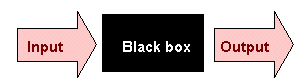
This form can be emulated on a spreadsheet, although the arrangement of the elements is not always so simple. (We are constrained by the technology.) We can think of four zones of a spreadsheet model as under.
| Zone 1 - Input variables |
| Key variables, especially those about which there is uncertainty. |
| Zone 2 - Manipulations |
| These are all the 'workings' of the spreadsheet. They may be in an area not immediately visible from the main screen. This is the model's 'black box'. |
| Zone 3 - Outputs |
| These are the outputs in which the decision-maker is interested. |
| Zone 4 - Graphical presentation |
| This is often a very useful and powerful way to add to understanding. Most spreadsheets allow us to display the graphs side-by-side with the data. |
Exercise
Develop a model to find the average per km cost of running your car. You have the following information:
Purchase price $25 000. It reduces in value in a straight line to be worth only $2 000 after 300 000 km (when it can be sold to a university student).
Gasoline consumption is 9.0 liters per 100 km. Gasoline price is 90 cpl.
Registration and third party insurance is $420 per annum. Other insurance is $300 per annum.
Tires cost $440 per set of four, and last 25 000 km.
Major service costs $360 every 20 000 km, minor service costs $120 every other 10 000 km.
Now you may not agree with these figures. Your Honda Legend may have cost $73 000, and you may know someone who can get you a set of tires in a cash transaction behind the Northern Cross Club for $280. But set the model up using the above figures; you can plug in your own figures later. You will need to take care with units - dollars, cents, thousands of km etc. Make sure your answers align with common sense - it doesn't cost $2.70 a kilometer to run a 1988 Toyota.
What we have not specified is the distance you travel each year. You may set up your output as a table - say 5 000, 10 000, 15 000, 20 000 and 25 000 km. See the sheet ch05ex04.xls for one way you may develop a model. (Note that to refer to the reduction in value averaged over the life of the car we have used the term "wear" to distinguish it from the financial accounting notion of depreciation.)
Once you have developed a model you may like to play with it. Put in your own figures. Test it to see what are the important items in car running costs. Then ask yourself what is a reasonable rate of reimbursement per kilometer for someone who uses a car for their employer.
Note that in response to the question "how much does
it cost you to run a car a kilometer?", the answer is a model, not a single bottom
line answer. You may want to come back to this model again when you look at cost/volume
relationships and break-even analysis in Chapter 12. (In Chapter 13, on life cycle
costing, we will see how you can accommodate the time value of money into such a model.)
Difference equations underlie many models. They are a way of breaking up a system, sometimes a complex system, into many small components. In financial and economical modeling we generally use difference equations to model how a system behaves over time, breaking the time period into such small periods that the simplifying assumptions in our equations do not affect the final result materially. For example, in demographics, we may develop a population projection which assumes all births occur at one time in the year, an assumption which would not matter if we were making a 20 year projection. There are some error in using a "lumpy" equation to model continuous flows, but these errors are trivial if out time intervals are small enough.
We can think of a system at times T and T+1 as being
connected by a set of transformations, which will be small changes if our time intervals
are small enough. In general the equations we can use to model the changes are simple,
linear equations (although the final model may be far from simple or linear. Often they
are equations of the form Y = AX + B.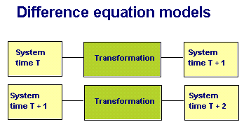
In modeling the behavior of a system over time we need to distinguish between stocks (a snapshot at a point in time) and flows.(what happens over time). The distinction is important, and is not always made clear in policy documents. For example, your income is a flow, your wealth is a stock.
That is, the value of a stock (YT+1) at time 'T +1' is related, by some flow, to the stock (YT) in the immediate preceding period (T). It's a simplification of many processes which occur continuously. For the sake of understanding, however, we break time into discrete intervals, to model a system into a series of interconnected stocks and flows. The systems at time T and T+1 can be modeled as stocks, and the transformations as a set of flows, usually related to the stock at time T. For example, Australia's population in June 2000 can be described as a stock (19.2 million people). The transformations can be modeled as a number of simple equations, describing births, deaths, and migration, which gives a net flow over the year. Births and deaths can be modeled by reference to the population in 2000; migration may be an independent variable. The 2001 population will be the 2000 population plus the net sum of these flows. And so the process repeats itself, with the opening stock of the next period being the closing stock of the previous period.
Once we have a set of starting conditions, and a set of simple equations describing transformations from one period to the next, then we can set up a spreadsheet model, along the general lines shown below.
| General Spreadsheet Model of a Difference Equation | ||||
| Parameters | ||||
| Time 0 | Opening stock | Transformations | Transformations | Closing stock |
| Time 1 | Closing stock from above | Transformations | Transformations | Closing stock |
| Time 2 | Closing stock from above | Transformations | Transformations | Closing stock |
Depreciation as Difference Equation
For example, refer to the declining balance depreciation model in Chapter 5, reproduced below.
| Example of Declining Balance Depreciation (25%) | |||
| Year | Book Value Beginning of Year | Depreciation | Book Value End of Year |
| 1 | 4 000 | 1 000 | 3 000 |
| 2 | 3 000 | 750 | 2 250 |
| 3 | 2 250 | 563 | 1 688 |
| 4 | 1 688 | 422 | 1 266 |
Note the "stocks" being the book values at the
beginning and end of year, and the "flow" being the depreciation. Note too that
the book value at the beginning of each year is equal to the book value at the end of the
previous year.
Another, slightly more complex model, is to model a tank as a system. Water flows into the tank at a rate 'I' liters per hour. It flows out at a rate 'O' liters per hour. The difference equation describing this system is:
QT+1 = QT + (I - O)
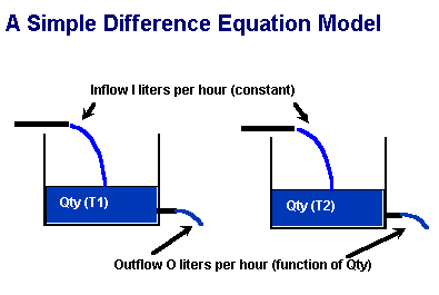 'I' may be steady, while 'O' may
be a function of Q. The more water there is in the tank, the more pressure there is to
sustain a flow. There may be an equation of the nature:
'I' may be steady, while 'O' may
be a function of Q. The more water there is in the tank, the more pressure there is to
sustain a flow. There may be an equation of the nature:
O = k * Qwhere k is a constant, which specifies the relationship between the variables Q and O.
There is a general five step process in developing adifference equation model:
Exercise
Model the tank using a spreadsheet. Assume the opening stock at time 0 is 5 000 liters, the inflow l is 1 000 liters an hour, and the outflow is 10 percent of the quantity - that is O = 0.1 * Q. Will the tank fill or empty, or will it come to some intermediate state?
The first few rows of the spreadsheet are shown below, A full model is at ch05ex05.xls.
| Spreadsheet Model of Tank | ||||
| Opening stock | 5000 | liters | ||
| Inflow rate | 1000 | liters/hour | ||
| Outflow | 10% | |||
| Time | Open | Inflow | Outflow | Close |
| 0 | 5000 | 1000 | 500 | 5500 |
| 1 | 5500 | 1000 | 550 | 5950 |
| 2 | 5950 | 1000 | 595 | 6355 |
| 3 | 6355 | 1000 | 636 | 6720 |
Equilibrium
Is there a stable equilibrium for our tank model? An equilibrium condition exists when there is no change from period to period. A stable equilibrium exists when the system always comes back to the same level following a minor perturbation.
First, let's calculate it mathematically. The equations describing the system and transformations are:
QT+1 = QT + (I - O) (Basic difference equation)
O = k * Q
Substituting for O in the above equation, we get:
QT+1 = QT + (I - k * QT)
QT+1 = (1 - k) * QT + I
Let's first see if there is an equilibrium condition, for which there is no change period to period - that is, QT+1 = QT.
QE = (1 - k) * QE + I
Expanding the brackets and rearranging:
QE - QE + k * QE = l
K * QE = l
QE = I/k
So much for the abstraction. That's a long-winded way of
saying that if water is flowing in at 1 000 liters an hour, and 10% is flowing out an
hour, it will stabilize at 10 000 liters. That's rather self-evident. It's hard to know
intuitively whether this equilibrium is stable, but a model can help us learn. Also, this
equation doesn't tell us how long the system will take to get to equilibrium, or how it
will behave on the way. The spreadsheet can help us answer those questions, and, besides,
it's simpler for those who don't like manipulating algebra.
Exercise
Using difference equations, develop a model of a financial investment accumulating compound interest. For starting values, assume an investment of $2000, and interest of 5 percent
This rate (5 percent) is around the accumulation you may expect to receive from a secure fund, such as a bank bill or cash management account. A diversified portfolio of equities will probably return about 10 percent over the long run in a combination of dividends and capital gains. Test your model with 10 percent and other rates of interest.
A spreadsheet is at ch05ex06.xls.
This is the familiar compound interest formula, which we'll meet again when we look at discounting in Chapter 9.
Exercise
Some people will take a lump sum on retirement, and will try to make it spin out over their remaining life. If you have a lump sum of $200 000, on which you could get a 6 percent return, and if you expect to live for 20 years (65 to 85), how much could you draw each year?
As a reality check, you know that the value has to be more than $12 000 (interest alone) and more than $10 000 (capital alone). But it cannot be as high as $22 000 (interest plus capital). It has to be between $12 000 and $22 000 - guess $17 000.
If you wanted to leave $10 000 to finance a wake, to what level would you reduce your annual drawing?
A spreadsheet is at ch05ex07.xls.
Exercise
In order to accumulate a lump sum, you will probably invest in superannuation. Develop a model, starting at age 35, finishing at age 65, with 7 percent interest, contribution of 12 percent of a $40 000 salary, and a 15 percent contribution tax each year. What will be the accumulation at age 55, 60 and 65?
A spreadsheet is at ch05ex08.xls.
You could easily combine these models to generate a complete lifetime superannuation plan.
A Warning on Models
Models are purposeful reductions of real systems. They incorporate simplifying assumptions. When the outputs predicted by models stray too far from our observations of real systems, our models need refining. This may sound self-evident, but there are many instances of policy makers placing too much faith in models, to the extent that they take on a normative dimension. (That is, they no longer describe how a system works, but how it should work, and if it doesn't work in that way there is something wrong with the system.) For an excellent description of how economic models have come to take on such a normative aura, see Brian Toohey's critique of economics - Tumbling Dice(3), and James Scott's Seeing Like a State.(4)
Specific References
1. Edith Stokey and Richard Zeckhauser A Primer for Policy Analysis (WW Norton NY 1978)
2. N Paul Loomba Management - A Quantitative Perspective (Collier Macmillan NY 1978)
3. Brian Toohey Tumbling Dice (William Heinemann Australia 1994)
4. James C Scott Seeing Like a State: How Certain Schemes to Improve the Human Condition Have Failed (Yale University Press 1998)