|
|
Queues are a part of life. On a holiday weekend in 1992 cars were piled up for three hours on the F3 freeway near Hornsby. We queue for a bus. We call a business and get treated to piped music while we wait in an invisible queue. Sometimes we are not aware we are in a queue; in a restaurant our order is in a queue while we are sitting at a table.
In discussing the theory of competitive markets, we showed how queues would not be sustained. If the price of a good or service were pitched too low there would be a queue for a while, but the market would interpret the queue as the need for a higher price. Price would rise, demand would fall, and the queue would disappear. In the longer term the higher price would bring forth higher supply and price may fall again. Similarly, if price were too high, accumulation of stock would lead to a downward adjustment.
But these adjustments are not instantaneous. Even in highly competitive markets queues form - try buying a pizza on the Monday night of a holiday weekend. It is particularly hard to balance supply and demand in the non-competitive situations in which governments operate.
Many government services are concerned with human service delivery. Queues carry human and political costs, as is evident from the ongoing controversy over hospital waiting lists, from the outcry when there are severe traffic jams, or from issues such as port congestion. In contrast, queues of inanimate objects in warehouses do incur costs (as we saw in Chapter 19 on inventory analysis) but, apart from the occasional complaint from accountants, they don't result in major political problems.
Queuing theory is a huge field, bringing together statistics, economics, and stochastic modelling. (Stochastic models are basically ones which rely on randomly generated statistical functions to simulate real life.) In this chapter we look at some aspects of queuing theory, including:
The main policy message is that even when we can calculate capacity requirements, by matching supply and demand through pricing or other mechanisms, there can be transient mismatches, resulting in queues or in unused capacity. These can come about from regular cyclical variations (e.g. morning and afternoon rush hours), from more random variations (e.g. weather patterns), or from some combinations of factors. As a general rule, because of randomness of arrivals, unless there is some queue there is likely to be unused capacity (a point often overlooked in the hospital waiting list debate).
If variations are regular and highly predictable we can develop simple deterministic models. If they are irregular and subject to random disturbances then our rigid computer models will not show up the temporary, random mismatches between supply and demand. We need to upset our models a little with random disturbances to emulate what happens in the real world. In this process we use random disturbances to produce reasonably predictable outcomes. For example, we can model with reasonable statistical accuracy what will happen at an airport with and without a new runway, through simulating variations in the arrival times of airplanes. The random inputs produce outputs which, while not deterministic, have a high degree of predicability for policy and planning purposes.
We conclude with a peek at chaotic systems - systems where
deterministic inputs produce seemingly random outputs.
The diagram below shows the basic elements of a process involving queuing.

It helps us to think about queues and their behavior if we think about each stage as having a defined process or discipline.
The arrival process can be random or structured. Often it is described in terms of the period between arrivals. It may have cyclical elements in it. No arrival process is 'pure'. Arrival of students for an oral exam would be highly structured, with evenly spaced appointments, but with some variation around these appointments, giving some degree of randomness. Within a short period arrival of customers at a bank may be random; over the course of a day it will have strong cyclical elements, such as the lunch time rush. The distribution of arrivals can sometimes be measured empirically. For new and unique facilities, such as the F5 freeway extension, it will be necessary to have a more abstract statistical model.
The arrival process may depend on some previous queuing process. Arrival of traffic at an intersection may be determined largely by the arrival of traffic at a set of traffic lights 500 meters back on the road. Arrival of passengers at customs depends on the immigration queuing process, which, in turn, depends on the airport flight queue processes. Queuing models can recognize this interdependence.
The queue discipline can be described in the same terms as are used in inventory models. We are most familiar with first-in-first-out queues (FIFO), as happens with lines at bus stops. Sometimes the discipline is last-in-first-out (LIFO), as may happen with a pile of student assignments or correspondence, where each new piece of paper is put on the top of the pile. There can be random service, as may happen in handing out relief food aid. There can be ranked queuing, with different customers being given different priority; this happens in emergency wards and in loading large airplanes. Sometimes there is mixed behavior, such as the refreshment stand during an intermission in a theater - elements of FIFO and random disciplines. Novel structures of queue discipline may elicit strategic behavior from customers, such as radio stations offering a prize to the sixth caller, or a customs inspector searching every third passenger.
There can be various combinations of queue and server. One queue one server is the simplest model, as with a breath test roadblock. (This also describes parallel independent queues, as once existed with bank tellers.) One queue multiple servers is now a typical situation in banks. Multiple queues single server is a possibility, as when two lanes of traffic merge into one. The discipline of multiple queues multiple servers often operates on turnpike toll gates and in McDonald's restaurants.
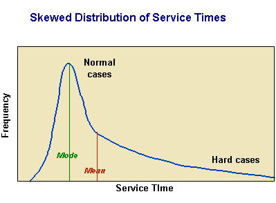
The service process, as with the arrival process, can usually be described in terms of some frequency distribution. The service time may be uniform or close to uniform, as with inoculations, or dishing out soup to a line of soldiers. Often it follows a skewed distribution, with a long tail, representing the harder cases. Most cases are routine, but some take a long time.
Supply-Demand Models of Queuing
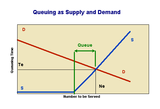
There can be interdependence between the three processes. If customers know of the queue, the arrival frequency will often be influenced by the queue length. The traffic helicopter in a busy city and the display lights in the reading room at the National Library are a form of negative feedback and therefore impose a stabilizing effect on queue length. In fact we can use standard supply/demand concepts to model queues. The figure below shows a pair of curves - a supply curve and a demand curve. The only difference between these and normal supply/demand models is that the Y axis on these models is in terms of time; the currency has changed from dollars to minutes. (This is a simplifying assumption, but it is necessary for a first order analysis because time is the currency of queues.)
For simplicity we can imagine a service which is "free" at the point of delivery - an attraction at a museum, a ride in an elevator. (For priced services, such as cinema admissions, we can consider the time cost of queuing and the financial cost of admission as separate, but interlinked systems). The supply curve of this system runs along the X axis, until all capacity is used. From that point, the kink in the curve, a queue develops, and the supply curve rises.
There is also a demand curve; different people have a different willingness to wait, as any parent knows. The value of the attraction and the cost of time differs between different individuals. When we combine the demand and supply curves, they meet, and that point of meeting is an equilibrium which determines the queue length and the waiting time (Te), just as in any other supply-demand model. If the queue length temporarily drops, more will join the queue; if it moves more slowly than expected, some will leave.
The Cost of Queues
Queues impose an obvious cost on customers. The most easily traceable is the waiting time, costed at some opportunity cost of time. Only if there is enough consumer surplus available will people queue, and the time spent in the queue is a diminution of this consumer surplus. In our model the rectangle formed by Te * Ne is the total "cost" of the queue, in terms of person minutes. This cost is economic waste, similar to deadweight loss, in that it is a payment without any beneficiary(1). It is likely to be very high for a unique or compulsory public service, such as mandatory vehicle inspection, The residual consumer surplus is given by the triangle between Te and the demand curve.
This deadweight loss can usually be eliminated by introducing a user charge, which can be modelled either by moving the demand curve down (obviously with a fee people will be less willing to spend resources queuing), or by moving the supply curve up (changing the Y axis from time to dollars). This second approach is modelled in the diagram. Note that the number served has fallen; Ne has moved to the left, and the cost has not fallen. It is, however, now a financial cost, which means that it transfers as revenue to the service provider. In an amusement park it may be possible to use this to reduce the admission charge; in government it may be possible to reduce taxes. In other words it may be possible to re-cycle the benefits; what is lost in consumer surplus can be returned in other ways.
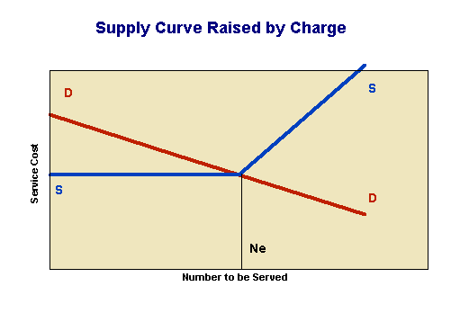
Fewer people use the service, as represented by the elimination of the queue, although just what will happen with throughput cannot be handled with this model. Does the facility close at a certain time, with all in the queue turned away, does the queue close earlier than the facility? They are the customers who valued the service the least, and they may share in some of the re-cycled benefits. For example, when a municipality starts to charge for use of public barbeques to eliminate queuing, it can reduce rates, or perhaps build more barbeques. The net social benefits are likely to be positive because of the elimination of unproductive queuing time.
Of course this is not to argue carte blanche for user pay pricing. If the price is set too high, or if the queue is only cyclical, there will be deadweight loss as the facilities lie unused because people cannot afford the fee. Also, setting a charging mechanism is costly; the transaction costs can be sufficiently high to offset much of the benefit of the pricing mechanism. One aspect of transaction costs rarely considered is the annoyance caused to customers in having to find small amounts of money, often in exact change (e.g. parking meters), and charging systems can introduce their own queues (e.g. lines to pay airport tax).
If demand is highly inelastic, then simply moving the supply curve up through user charges won't help, because the kink will remain to the left of the demand curve. In such cases the only way to eliminate the deadweight loss is to expand the service. For example, some user pay dogmatist on observing immigration queues at an airport may suggest an immigration processing charge. That would have no effect on queue length, and no reduction in deadweight loss.
This supply-demand model assumes all customers have the same value of time. If we change this assumption then it is possible that a user pay system will change the distribution of the service. Those who place a high value on their time will be more accepting of a user pay system, while those who place a low value on their time will favor queuing. Some people who could not afford the time to queue may be able to afford a user charge, and vice versa. At first sight this may appear inequitable, for we generally assume that the better-off have a higher cost of time. On reflection, this is not necessarily so. Old people may find it tiring standing in line. Someone with an expiring parking meter will find it very costly to queue at an ATM. You have probably had the experience of making an international or interstate call, and being placed on hold; you are paying dearly for your time, while the other customers are mainly locals. Perhaps, in time, someone will have the sense to program an option "if you would like to jump to the top of the queue, please press 1 on your phone, and your account will be debited $1".
This equilibrium analysis assumes, as do other economic
equilibrium models, perfect knowledge. Often customers cannot make a rational choice; they
misjudge the length of queue. At Disneyland, for example, the waiting areas are designed
so that customers don't see the full length of queue; by the time they turn the first
corner and see the queue is twice as long as they thought, the time spent so far is a sunk
cost - the customer may as well stay in the queue, even though he or she would not have
joined it in the first place. As yet, few telephone queuing systems offer any feedback on
queue length.
Interdependencies of Processes
The supply/demand model uses conventional economic analysis to show that a queue could come to an equilibrium. It incorporates the normal economists' assumption that supply and demand are independent.
Supply and demand are not necessarily independent. They can, in some cases, interact to produce positive feedback or destabilizing effects. If fans for a once-only rock concert think there are plenty of seats, no queue is likely to form. If, however, the word gets around that seats are in short supply, an all night queue may develop on the pavement outside the ticket office. Thomas Schelling describes such phenomena through the musical chair metaphor.(2) The existence of a queue may stimulate demand; if it's worth queuing for it must be good! While normal negative feedback processes can be modelled, these positive feedback systems are very hard to model - small perturbations in expectations can result in a long queue suddenly appearing, especially if demand is highly inelastic, as for trivial events like rock concerts and serious events like getting a place on an aircraft out of a war zone.
Service time may be a function of queue length; as the queue gets longer service may speed up. Public servants clearing backlogs of correspondence know this process. This has a stabilizing effect on the process.
There can be more complex interdependence when queues operate in a closed system. Thomas Schelling describes a ski slope with a single ski lift, with a line of skiers waiting to get on the lift. To shorten the queue the operator of the lift speeds it up. At first sight we would think this shortens the queue.
The effect is counter-intuitive, until we think of the
system as a closed one. Skiers spend their time doing one of three things - coming down
the mountain (a constant), standing in line and going up the mountain. If skiers spend
less time in one of these three states they will spend more time in another. This is a
metaphor for that part of hospital waiting lists composed of people with multiple
conditions or the need for frequent follow-up services.
If we know demand (the arrival process) for a service with
near certainty we can develop deterministic models of a queuing process. A deterministic
model is often a useful first step in designing a new facility.
Exercise
A new bridge is to be built to replace an aged structure. There is no easy alternative route. The project will be financed by a toll. Each tollgate can handle 2000 vehicles an hour, or 48000 a day. Traffic demand is as under:
Period |
Arrivals | Period | Arrivals |
Period | Arrivals |
| 0000-0100 | 1 000 | 0800-0900 | 10 000 | 1600-1700 | 10 000 |
| 0100-0200 | 700 | 0900-1000 | 9 000 | 1700-1800 | 12 000 |
| 0200-0300 | 500 | 1000-1100 | 6 000 | 1800-1900 | 10 000 |
| 0300-0400 | 300 | 1100-1200 | 6 000 | 1900-2000 | 6 000 |
| 0400-0500 | 500 | 1200-1300 | 6 000 | 2000-2100 | 4 000 |
| 0500-0600 | 1 000 | 1300-1400 | 6 000 | 2100-2200 | 2 000 |
| 0600-0700 | 2 000 | 1400-1500 | 6 000 | 2200-2300 | 2 000 |
| 0700-0800 | 4 000 | 1500-1600 | 8 000 | 2300-2400 | 2 000 |
| Total over 24 hour period | 115 000 | ||||
The task is to model the effects of various numbers of
tollgates. It is obvious that with 3 tollgates, providing capacity for 144 000
vehicles a day, the traffic will clear over a 24 hour period, but how long will the queues
be? It is also obvious that with six tollgates the afternoon peak can be accommodated with
no delay. What is the effect of having various numbers of tollgates?
The spreadsheet is at ch20ex01.xls. To construct it requires handling a little Boolean logic, which is easy enough, but the prime purpose is to show various approaches to modelling. (The exercises in this Chapter give only the completed models.)
Note that as the problem is structured it is
deterministic; one model will give one clear answer. We break from that assumption with
the next two exercises.
Stochastic or probabilistic models can get very complex.
The two exercises that follow take two simple situations and develop simple probabilistic
models. In both cases we assume simple queue discipline and a one queue one server system.
We assume service time is constant, but build the randomness into the arrival process.
Exercise
A health department intends to operate a sexually transmitted diseases clinic. To maintain informality and confidentiality there is no appointment schedule. It operates on a walk-in basis. Its front door is open for 8 hours every day, and each customer takes ten minutes to attend to. It thus has the capacity to serve 48 customers a day. Once customers have been admitted to the waiting room all are attended to, regardless of how many are in the waiting room when the doors close.
On average one customer comes every ten minutes; it is operating at capacity.
We need to know how long we will have to keep the clinic operating once we have closed the front door. We also may need to know how long the queues are likely to get, so that we can design a waiting room.
Now the arrival processes are random. We know the average over a long period, but we don't know how many customers will come in any one ten minute period.
Those who have studied statistics will recognize here a Poisson distribution, with = 1.0. (3) We can understand the distribution with a simple metaphor. Imagine there are 365 people in a room. What is the probability that today there will be n birthdays?
The Poisson distribution in the birthday case is shown below:
| Number of Birthdays Today | Probability | Cumulative Probability |
| 0 | 0.3679 | 0.3679 |
| 1 | 0.3679 | 0.7358 |
| 2 | 0.1839 | 0.9197 |
| 3 | 0.0613 | 0.9810 |
| 4 | 0.0153 | 0.9963 |
| 5 | 0.0031 | 0.9994 |
We could continue the table all the way up to the possibility
that there are 365 birthdays today. By going to five, however, we have covered 99.94
percent of possibilities. If we multiply out the probability by the number of birthdays
and add the result then we find the average number of birthdays in any one day is one.
The same table can be used for the STD clinic.
In the spreadsheet ch20ex02.xls random numbers are used to look up how many people will come through the door. The random number function in computers returns a number between 0 and 1, evenly spread over that range. We have programmed the spreadsheet using the <Lookup> function so that in each period we select a random number. If it is between 0.0000 and 0.3679, then no customers come in. If it is between 0.3679 and 0.7358 (the cumulative probability), then 1 customer comes in. If it is between 0.7358 and 0.9197, then 2 customers come in, and so on.
The result is in the spreadsheet. This time it is not
deterministic. If one (or a group) repeats the modelling enough times, then it is possible
to build up a distribution of results for the number waiting at the end of the 12 hour
period and the maximum number in the queue. (A hint on stochastic modelling using random
numbers - to recalculate a new condition in most spreadsheets press the <F9> key. )
Exercise
Stochastic modelling is of most interest when systems are operating near capacity. If there is plenty of capacity, then queuing isn't a problem (but efficiency is). If the system is operating at full capacity, and queues have stabilized, then the problem is usually self-evident.
Imagine an airport with flights scheduled to arrive every six minutes. It is operating at capacity, because it takes six minutes to clear the runway and allow another plane to land.
Now even though there is discipline on the airlines to plan their arrivals, flight crews cannot plan precisely; flight arrivals are distributed normally around their planned arrival time with a standard distribution of two minutes. The distribution is shown in the diagram below.
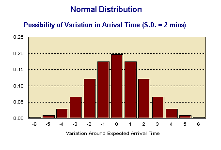
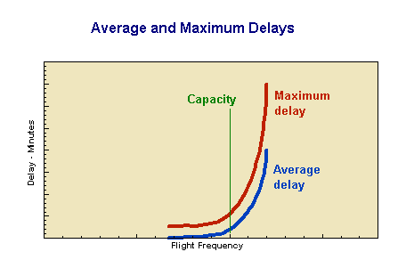
Again we can model this situation, using the same basic logic as we did with the STD clinic above. We can model this system at various arrival intervals, and see what sort of distribution of average and worst delays we get as we move up through and past capacity The spreadsheet at ch20ex03.xls is set up for 96 flights - equivalent to about ten hours of busy operation.
We should get a graph like the one alongside - where the lines are measures of central tendency. The main message is that capacity problems creep up on us. The situation gets worse only slowly at first. In any system 'capacity' is not a brick wall; rather it is something we approach and pass through, with rapidly worsening queues. This graph is similar to the theoretical kinked "supply" curve developed earlier; randomness in the system has smoothed out the kink.
In our modelling we have developed systems which are either deterministic or are non-deterministic but with reasonably predictable outcomes.
We hinted at highly unstable systems when we mentioned positive feedback earlier in this chapter. The queuing models for the rock concert, for relief flights out of a war zone, may be chaotic - essentially indeterministic because of highly amplified effects of tiny variations - a rumor here, a false report etc.
In ch20ex04.xls we have modelled a very simple difference equation:
Value T+1 = Constant * Value T * (1 - Value T - 1)
The constant is called the gain of the system. This difference equation is a model of certain forms of biological reproduction. At very small levels of gain it describes a system moving into extinction. As gain increases it describes systems moving to a new steady state. Then as gain increases further it describes systems which become chaotic - indeterminate. At higher levels of gain chaos gives way to systems which rapidly move to infinity.(4)
We have illustrated the system at a gain of 2.7, which shows a system which overshoots and oscillates a little before settling down.
To manipulate the model load the spreadsheet and vary the gain. The results are interesting! Try the equation on different software - the result may be different because of minor computational differences between different spreadsheets.
Even simple sets of variables can produce highly indeterministic outcomes. How much harder it is to model complex systems, or to attempt to use high-gain systems like monetary policy to stabilize an economy. Economists working with chaotic models are re-interpreting systems which they once saw as deterministic (e.g. cyclical) as being chaotic. If such a simple equation can give such unpredictable results, then how much more complex is the task of interpreting the driving forces in a real-world system and of designing stabilizing interventions.
General References
Edith Stokey and Richard Zeckhauser A Primer for Policy Analysis (Scott, Foreman and Co 1987)
Specific References
1. Some writers, such as Edith Stokey, do call this deadweight loss.
2. Thomas Schelling Micromotives and Macrobehavior (W W Norton NY 1978)
3. Taro Yamane Statistics (Harper and Row 1967)
4. An excellent introduction to chaos theory for the non-mathematically inclined is James Gleick Chaos (Cardinal London UK 1987)