|
|
In the mythical thing called a perfect market, there is no pricing decision to be made. Suppliers take the price set by the market's 'invisible hand'. If the price of tomatoes is $2.75 per kilo, then the stallholder who marks them up to $2.85 will lose all custom to the next door stall. By marking them down to $2.65 the stallholder will sell plenty of tomatoes, but won't be able to afford to stay in business long, because revenue won't cover expenses.
Economic teaching focuses largely on the operations of the competitive market, with a heavy emphasis on the workings of the perfect market in which there is perfect competition. It's a market with many suppliers, many buyers, no collusion, and a free interchange of information about prices and non-price factors such as quality. There are examples which approximate a free market - gasoline retailing in a big city, fruit and vegetable markets etc.
At the other extreme is monopoly. That is where there is one supplier and many buyers. Popular writers weave stories about the injustices of monopoly. Economists use monopoly as an analytical tool, pointing out how monopoly is not only unjust but also inefficient. As with perfect competition, pure monopoly is hard to envisage. BHP may dominate domestic steel production, but there are imports to keep prices checked. The ACT Electricity and Water Authority may be the only electricity company in Canberra, but there are substitutes for electricity in many applications, and consumers will turn to them if ACTEW sets its prices too high.
Markets are not essential for economic activity; many transactions take place without formal markets - redistribution within a household, voluntary work etc. For an erudite treatment of non-market transactions see the writings of economic philosopher Karl Polanyi.(1) This, and the following chapter, however, are confined to market transactions - first in competitive markets and then in monopoly situations.
Monopoly and competition are pure models, useful for analytical and learning purposes, but they are rarely descriptive of anything we see in the world. A common situation is oligopoly, where there are few suppliers but many buyers. We see this situation often in a small economy like Australia. Airlines are a case in point, and much of the liberalization over the eighties was aimed at breaking up oligopolies such as banking. The 'few' suppliers need not be small in number; they may be disciplined by strong anti-competitive behavior, as is the case with lawyers and medical practitioners.
Another situation, often by-passed in text books, is monopsony,
where there is one buyer and many suppliers. It's often faced by small farmers selling to
one processor or distributor. And then there is the common case of
monopolistic competition, in which firms use various means - advertising,
product design, special features - to differentiate their products from those of their
competitors.
Before going into details of public intervention in the
case of market failure, which we look at in Chapter 16, it is
worth reviewing the main characteristics of markets - looking at supply,
demand, how they interact, the notions of supply, demand and
income elasticity, and the notion of surplus.
This is a cursory treatment of market theory; students are advised to follow through by
referring to a text on microeconomics for a more complete treatment of market theory.
Supply
The key theory of supply is that higher prices bring forth higher supply. If we consider price as an independent variable, then the higher the price the higher will be supply, as existing producers expand and as new producers enter. The key concept is that in a profit-maximizing enterprise, production expands to the point that marginal cost equates to, or does not exceed, marginal revenue. Conceptually, marginal revenue is just like marginal cost - it is the revenue on the last unit sold. In Chapter 12 the power generating utility we modelled has a marginal cost (at 35 GwH) of 3.5 cents a unit, and can get 8.0 cents a unit from customers. Imagine it has an opportunity to sell some power, through the national grid, to an adjoining state, but it must take a discount to 6.0 cents, because of transmission losses. It is still profitable to supply this market, for a marginal revenue of 6.0 cents and a marginal profit of 2.5 cents. It would still be profitable to supply a more distant market where it could get only 3.6 cents.
As an example to illustrate the theory in this chapter, imagine we are running an 'in house' print room in a government agency. It has fixed costs, including a reasonable return on invested funds, of $400 000 a year, and a 'U' shaped marginal cost structure. Initially as volume expands it can use its machines more efficiently, and obtain discounts on paper and inks. However, as output expands further it has to rely on overtime, to use machines sub-optimally, and to swing older machines into production. Its marginal cost structure is as under:
The print room is entirely a price-taker. If price rises it will adjust its supply accordingly.
We can develop a model of this enterprise. At the simplest level, however, we can see that at prices below $35 it will probably not supply at all. What's the point if it cannot cover its variable costs? In fact we can calculate that the price must be at least $40 for this enterprise to cover its variable costs, and we can calculate a table as set out below.
| Price ($/'000) | Vol (million) | Profit $'000 |
| 0 | 0 | -400 |
| 10 | 0 | -400 |
| 20 | 0 | -400 |
| 30 | 0 | -400 |
| 40 | 0 or 15 | -400 |
| 50 | 20 | -225 |
| 60 | 20 - 25 | -25 |
| 70 | 25 | 225 |
| 80 | 25 | 475 |
| 90 | 25 - 30 | 725 |
| 100 | 30 | 1 025 |
| 110 | 30 | 1 325 |
| 120 | 30+ | 1 325 |
| 130 | >30 | >1 625 |
The profit figures cannot be obtained without constructing a model; they are included in the table only for completeness. (The model is at ch14ex01.xls) The volume figures below a price of $35 are obvious - supply is zero. Between $35 and $45 we have to interrogate the model to see whether it is worth going ahead and producing - can the print room cover its variable costs? (In fact, at a price of $35, for example, it would be better off not to produce at all, and at a price of $40 the decision whether to run or not would be touch and go.) From there, however, it's obvious that the print room will maximize its profits (or at least minimize its losses) at a point just before marginal cost rises above the price it can receive for its output. It will expand its output up to a point where marginal cost = marginal revenue. As long as the firm can get a profit on the last unit sold, no matter how small, it will sell it.
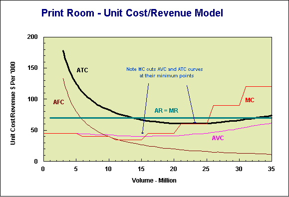
The graph below and the spreadsheet from which it is derived illustrate, as an example, the print room in a situation where it can sell its output for $70 per thousand sheets. At that point the MR curve (the $70 straight line which is also the average revenue) crosses the MC curve (the light solid line) at a volume of 25 million. To go beyond that point the enterprise would incur a marginal loss. (It could still make an absolute profit up to a volume of 32 million, where the ATC curve crosses the AR curve, but at this point there would be no profit left. The losses on the production between 25 and 32 million would have wiped out the profits on production between 14 and 25 million. As that MR curve moves up, as a result of plugging higher prices into the model, it intercepts the MC curve at higher and higher volumes.
As a general rule, higher prices bring forth
higher supply. This holds for this print room and for the whole industry; as prices rise
new entrants, attracted by the profits to be made, open up production and start to supply
the market. (Perhaps some are old producers who have had their equipment mothballed.) At
low prices, such as $50, printers will continue to supply for some time, but eventually
will close down when their 'fixed' costs become 'variable' or discretionary - what
economists call the long run, when they make decisions like
whether to replace aged equipment, to renew a lease, or to take on another apprentice.
Supply and Elasticity
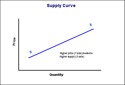
The general relationship between price and quantity supplied can be plotted graphically. Here we will have to bear with a convention of economists; they put price, the independent variable, on the y axis, and quantity, the dependent variable, on the x axis. This gives a supply curve, with a slope upwards to the right.
The shallower that slope, the more responsive is supply to price. The technical term for this responsiveness is supply elasticity. It is measured mathematically as:
(percentage change in supply)/(percentage change in price)
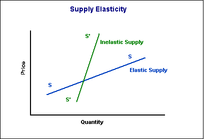
Elasticity is high in markets where supply can be changed quickly, or where supply from stock is possible.
Unskilled labor and industries employing unskilled labor
may be able to change supply very quickly. Some farm industries, such as dairying, where
many costs are fixed and capacity takes a long time to change, can change supply only very
slowly. In some markets, such as foreshore land on Sydney Harbor, total industry supply is
close to entirely inelastic - a point we may have noted when we looked at real price
movements in Chapter 7.
Lowest Cost Supply
In our print room example, as prices rise, initially existing printers will do better and better. Eventually, however, the word will get around that there are profits in printing, and more printers, attracted by the prospects of profits, will enter the market. (In economists' terms there will be a shift outwards of the supply curve.) With the increasing supply, prices will eventually come back, until all excess profit (economic profit) is wiped out. This is shown graphically on the next page.
There is a period of profit, which, in the case of industries with a slow response, may last for some time, until the industry expands to absorb the higher demand. Sometimes the industry over-expands, and the result is an ongoing cyclical behavior, the stable zero profit price being something firms meet only on the way up or on the way down.
If the new entrants to the industry have a lower average cost, as they may have if they use different technology, or if they are not bound by contractual labor arrangements, the final price will be lower than the initial price.
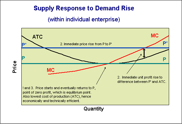
This model as an equilibrium one. If the
price is greater than P then new entrants will come in and will undercut the firms which
are operating uneconomically, pulling price down. If the price is lower than P, then all
firms will suffer negative (economic) profits, and some firms will go out of the business,
thus allowing a price rise among the survivors.
Exercise
Assuming all print operations have the same cost
structure, what will be the price which will provide exactly zero profits? (Remember that
a reasonable return to capital is included in 'costs'. ) You can find the answer
mathematically, but it is most easily found by constructing a spreadsheet, 'plugging in'
various prices, and at each price finding a maximum profit, or minimum loss. There will be
one price where there is exactly zero profit.
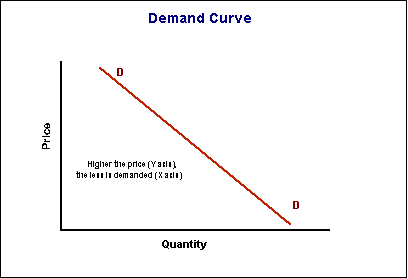
The other side of the basic economic relationship is demand. Generally, the higher the price for any good or service, the lower will be demand.
Thus we get a demand curve which is like the supply curve but sloping in the opposite direction.
The demand curve can be ascertained by market research, using questionnaires, or techniques such as looking at past levels of demand in response to different prices. For example, over the mid-seventies and early eighties the wholesale price of beef in Australia was around $9.00 per kilo (1995 prices) and average per capita consumption was around 45 kilos a year; in the late seventies prices fell to around $6.00 per kilo and consumption rose to around 65 kilos. Such analysis gives us an individual demand curve; the industry demand curve is the horizontal summation of 17 million such individual curves. In a competitive market, however, each producer faces a 'flat' demand curve. His or her influence on the market is infinitesimally small - the beef producer, selling 400 cattle a year, sees only that part of the industry demand curve, say, between 9 999 600 and 8 000 000 in a market of 8 million cattle.
As with supply, there is also the concept of demand
elasticity (more fully price elasticity of demand),
which measures the responsiveness of demand to price. In the case of beef, a 33 percent
decrease in price brings forth a 44 percent increase in consumption. This implies a demand
elasticity of -1.33 (note the negative sign, and note that the precise measure will depend
on the point from which we start to measure(2).)
Exercise
The passenger ferry between the mainland and Porcupine Island costs $150 000 a year to run, regardless of passenger numbers, and has never broken even. Market research suggests the following passenger numbers at various fare levels:
| Fare | Passengers |
| $1.50 | 60 000 |
| $2.00 | 50 000 |
| $2.50 | 40 000 |
| $3.00 | 30 000 |
The state finance department has suggested that the fare should be raised to the point of
full cost recovery. What is an appropriate response to this suggestion?
If an enterprise is not simply a price taker, but has the capacity to set its prices, then it starts to suffer a loss of revenue once it pushes prices to the point that demand elasticity is below -1.0. If its variable costs are high it may suffer a decline in profit well before this point, but frequently, in government monopolies, variable costs are low, and profits are closely related to revenue. The key assumption in economic models is that firms seek to maximize profit, rather than revenue. Pursuit of other objectives is explored in the next chapter.
Demand elasticity depends on whether the good or service is a necessity or not. If it is not particularly important in one's consumption, or has close substitutes, then elasticity will be low. Demand for beef will depend not only on its own price, but also on the price of mutton and fowl, for example. Demand for specific goods is more price elastic than demand for generic goods. Demand for Wolf Blass Rhine Riesling is more elastic than demand for Rhine Riesling which is more elastic than demand for white wine, which is more elastic than demand for wine .....
Another economic concept is income elasticity
of demand. For most goods, the higher our income,
the higher is our consumption. For inferior goods income
elasticity of demand is less than 1.0. That is, the higher our income, the less we consume
as a proportion of our income. Most goods and services fall into this category. Some goods
and services are superior goods, for which consumption rises
more quickly than income. An analysis of Australia's household expenditure data reveals
very few such goods - glassware, music disks, and urban rail and ferry fares.
Demand Elasticity and Indirect Taxation
Governments impose sales taxes for two reasons. The main reason is to raise revenue. (Sometimes, but not frequently, this is dedicated to a specific use, a hypothecated tax, as with the NSW fuel levy, but most often it is designed simply to raise general revenue.) The other reason, infrequently applied, is to discourage consumption, and we are, perhaps, seeing a change in treatment of cigarette taxation. If demand elasticity is high enough, then an increase in tax will actually result in a decrease in revenue. (This is illustrated in the Taxation Section, in Chapter 2.)
This is why governments do not go all out taxing luxury items; they don't want to erode their tax base. Australia's highest sales tax rates are on electronic goods and perfumes, not because they are 'luxuries' (though this may be the political rhetoric), but because demand is reasonably price inelastic.
Because of substitutability, there is a case for keeping indirect taxes broad; different taxes on substitute goods will distort consumption choices. We now have many highly differentiated taxes on goods with close substitutes, for example fruit juice and fruit. This is why there is a case for broadening and simplifying the indirect tax base.
Equity considerations suggest that sales taxes will be
most regressive if applied to goods and services for which income elasticity is low.
Research for the Australian Consumers' Association reveals that there are many high taxes
on items with low income elasticity. For example there are high Commonwealth sales taxes
on household appliances and television receivers, high state charges on motor vehicles in
the form of registration fees, high state land taxes which are passed on to rental
tenants, and monopoly profits from electricity.(3)
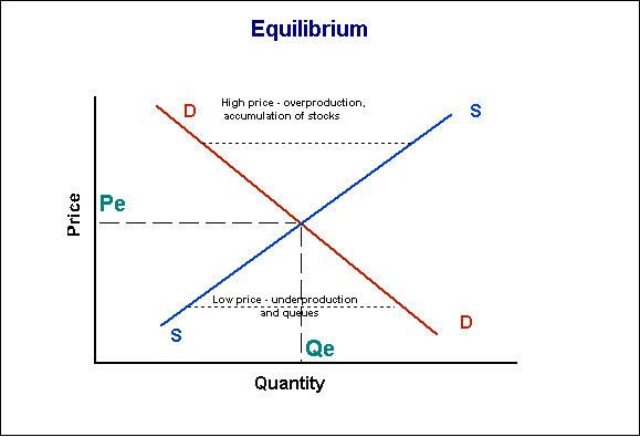
So far we have considered supply and demand in isolation, and have treated price as something of an exogenous variable. In the economic model of markets, price is set by the market. In economic theory price comes out of the interaction of demand and supply, not from one or the other.
The market-determined price Pe is at the intersection of the supply and demand curves. Look at the figure below. It's not immediately obvious why Pe should be the market-determined price, but imagine what would happen if price were at some other level.
If price were above Pe' there would be extra supply, and there would be reduced demand. Firms would be producing more than customers would be willing to buy - stocks would be accumulating. This is essentially what happened with wool in Australia up to 1991. Eventually prices would have to drop to clear stocks. The high price both suppresses demand and increases supply, exacerbating the stockpiling problem.
If price were lower. then production would be insufficient to meet demand. The signals of low price would bring forth more customers, but insufficient supply to meet the demand. Queues would form, as happens when there is rent control, or end-of-year bargain sales.
The price Pe is an equilibrium price. Any disturbance from this level and there will be forces to restore it. That is the essence of the economic model of supply and demand.
Surplus and Deadweight Loss
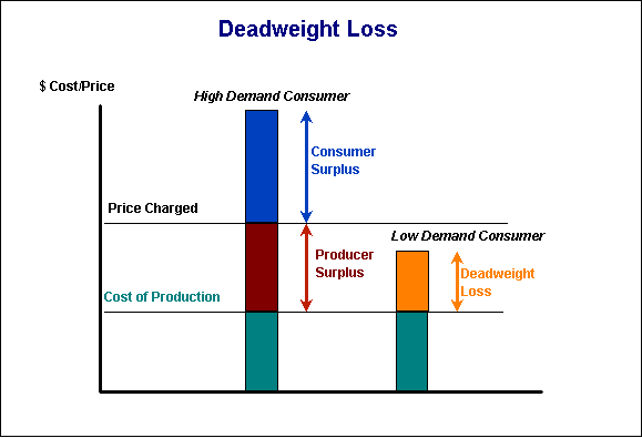
Economists talk about producers' surplus, consumers' surplus and deadweight loss. The concepts might sound mysterious, but they are simple and well known in everyday life.
Imagine you've been on a seven day backpacking expedition which lengthened to nine days because of foul weather, and are just coming into civilization - a kiosk at a trail head. You haven't had a warm drink in two days, your clothes are wet through, you have had nothing but muesli and water for three days. You do have $100 in your pocket to spend on luxuries when you come out.
You notice at the trail head that they sell coffee for $5.00 a cup. You know it costs only about $2.00 (ATC) to make, but you are so desperate you would give $10.00 for a cup of coffee.
Now the difference between $10.00 you are willing to pay and the $2.00 production cost is the surplus available for distribution between the producer and consumer. If you pay $5.00 there is a $3.00 surplus for the producer and a $5.00 surplus for the consumer. You may feel ripped off, but you will also feel warm.
In a competitive market all the surplus accrues to the consumer. Think back to the print room example, where we saw profits eroded back to zero. In a monopoly, however, much or all of the surplus may pass to the producer, and some transactions that could have been beneficial to one or both parties may not take place at all. That's the problem of deadweight loss. Your companion on the walking trip would like a cup of coffee too, but not being so desperate is willing to pay only $4.00 for it. There will be no sale because the price is $5.00. There could have been a distribution of the surplus of $2.00 between the consumer and producer, but no transaction takes place.
The situation of the two consumers is illustrated in the chart below. The consumer willing to pay more, the high demand consumer, shares surplus with the producer. (In a competitive market all surplus would be consumer surplus, as the price would be the cost of production.) The consumer willing to pay less than the price charged, but still willing to pay more than the cost of production, the low demand consumer, does not buy, and there is deadweight loss.
These concepts of consumer surplus and deadweight loss are covered in more detail in Chapter 15 on monopoly, where we see how surplus is appropriated not just as producers' profit, but also as transfers to other parties. Chapters 15 and 16 also look at look at public policy options in situations of natural monopoly.
General References
Most of the theory in this chapter can be found in a good economics text.
William C Apgar and H J Brown Microeconomics and Public Policy (Scott, Foreman and Co 1987)
Specific References
1. Karl Polanyi The Great Transformation Beacon Press 1944
2. Strictly, elasticity should be measured at a point; it is a differential concept. Practically, however, it would be impossible to make any empirical measure around a point.
3. Ian McAuley Consumption Tax - A designers Guide to Consumption Tax (ACA Policy Discussion Paper 1991)