|
|
There are many financial and economic problems involving optimization. The most general is one of maximising profit. Public sector agencies will have more complex objectives generally, but still the issue of optimization arises.
In general, we can optimize on only one variable at a time, but we often forget that general rule. For example, common terminology is often to refer to 'the best and fairest football player'. A moment's reflection will show that these two qualities probably involve some trade-off, and are unlikely to be found in the same person. Some years ago a Deputy Secretary in the Department of Trade and Industry, writing a speech for the Minister, stated "Australia's trade objective is to maximize the value and volume of its exports." The speech made it through all the scrutiny of the Minister's office and was eventually delivered. Issues of optimization, including the general rule that we can usually optimize on one variable at a time, are not always self-evident.
Inventory management is an example of a class of problems in which we seek to achieve an optimum, to minimize the costs associated with holding and re-ordering stock.
In general, the more inventory we hold the more we have to pay to finance that inventory. The notion of the accountant wandering the warehouse, distressed at the level of stocks, is a familiar one. The accountant, struggling with an overdraft, sees money tied up in stocks. The more stock we have the more spoils, the more storage we need, and the higher is the risk of obsolescence.
On the other hand, the lower the level of stock we hold,
the more often we have to replenish it. In a manufacturing operation producing a run may
involve high setup costs. In a non-manufacturing operation, such as a hospital pharmacy,
there is still a significant cost per order - raising an order, entering the transaction
into the accounts, checking the consignment, unpacking, etc, as well as the risk of
running short of crucial supplies.
There is an optimum point for stock
replenishment, and we can most easily illustrate it by developing a stockholding model.

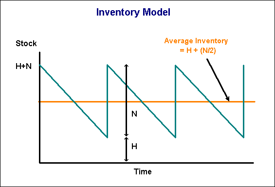
If H is the minimum permissible stock, N the size of the production run or order quantity, F the fixed cost per order, v the unit variable cost (usually AVC), and R is our annual usage, then we can develop a model using these variables.
First, our inventory over time will be a sawtooth function, as illustrated above. When the inventory gets down to H we restock with N units. A uniform drawdown produces a straight line falling away from H+N to H, at which stage the stocks are replenished. (In this case we've assumed instant replenishment, but a build-up could be accommodated.)
With a uniform drawdown the average stockholding is H + (N/2), as shown in the diagram above.
We can look at two elements of costs - re-ordering costs
and holding costs.
Re-ordering Costs
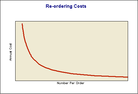
If we use R units a year, then we will place R/N orders a year. If each order costs us F dollars, then our annual re-ordering costs will be F*R/N.
This is a function which looks like the one below.

Holding Costs
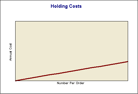
The holding costs will relate to the average value of stock.
The average level of stock is H + (N/2). Its value is v * (H + (N/2). The holding cost is:
i * v * (H + (N/2)).
That is:
(i * v * H) + ( i * v * N/2)
The left hand term is outside our control, and is independent of N. It needn't enter our consideration further.

Combined Costs
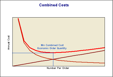
We want to minimize the function:
(i * v * N/2) + (F * R/N)
This combined function will be U shaped, with a minimum point.

The actual calculations we can do in one of two ways. One is with a spreadsheet and the other is with algebra.
We'll illustrate the spreadsheet method with an example,
and then construct the general algebraic solution.
Spreadsheet Solution
Imagine a hospital pharmacy with the following salient cost structure for a particular pharmaceutical:
Fixed cost per order (F) $80
Unit variable cost (v) $200
Annual usage (R) 120 prescriptions
Real interest rate (i) 8%
We don't need to know the minimum stock size.
We can set up a spreadsheet as below. (ch19ex01.xls) We can see that the optimum order quantity is 35 units.
Included in the spreadsheet are marginal cost figures. An alternative way to envisage this problem is to think of increasing the re-order quantity until the marginal reduction in re-ordering costs comes down to meet the marginal increase in holding costs. The marginal re-ordering cost falls away with the number ordered, and crosses the marginal holding cost ($8 per unit) at the point of minimum combined cost.
| Number in each run (N) | Re-ordering costs | Holding Costs | Combined Costs | Marginal Re-ordering Cost | Marginal Holding Cost |
| 0 | |||||
| 5 | 1920 | 40 | 1960 | ||
| 10 | 960 | 80 | 1040 | -192.00 | 8.00 |
| 15 | 640 | 120 | 760 | -64.00 | 8.00 |
| 20 | 480 | 160 | 640 | -32.00 | 8.00 |
| 25 | 384 | 200 | 584 | -19.20 | 8.00 |
| 30 | 320 | 240 | 560 | -12.80 | 8.00 |
| 35 | 274 | 280 | 554 | -9.14 | 8.00 |
| 40 | 240 | 320 | 560 | -6.86 | 8.00 |
| 45 | 213 | 360 | 573 | -5.33 | 8.00 |
| 50 | 192 | 400 | 592 | -4.27 | 8.00 |
| 55 | 175 | 440 | 615 | -3.49 | 8.00 |
| 60 | 160 | 480 | 640 | -2.91 | 8.00 |
| 65 | 148 | 520 | 668 | -2.46 | 8.00 |
| 70 | 137 | 560 | 697 | -2.11 | 8.00 |
| 75 | 128 | 600 | 728 | -1.83 | 8.00 |
| 80 | 120 | 640 | 760 | -1.60 | 8.00 |
This suggests a regular re-stock in the order of 35 units.
Note that the penalty for erring on the low side is much higher than the penalty for
erring on the high side.
Algebraic Solution
The task is to minimize the total cost function:
C =(i * v * N/2) + (F * R/N)
The general condition for a minimum is to find the turning point, which is where the partial derivative (with respect to N in this case) is equal to 0.

Plugging our values for F, R, v and i into the above equation gives N = 37 units, which is slightly more fine-tuned than the spreadsheet solution (which was in steps of five).
The algebraic solution is faster, in that it doesn't require us to set up a spreadsheet. But it's more of a black box, with workings not evident to the decision-maker. It is, therefore, less convincing.
Also, we can incorporate more elements into our
spreadsheet. It may be that we can get a discount for orders of more than 20 and 40 units.
These non-continuous functions are easy to incorporate into a spreadsheet. They cannot be
represented by a single equation.
Uses and Limitations of Inventory Models
The model above is useful in bringing some rationality into a system which is often dominated by short term cash considerations. Re-ordering does involve costs, and not all of these costs are easily traceable. Also, looking at the curves, the cost of being on the high side of the optimum is generally less than the cost of being on the low side.
The model above does not measure all the costs of holding stock. It would be easy enough to modify it to build in physical carrying costs, such as rent of storage space and insurance of stock. (This simply becomes another function dependent on N, probably linearly variable.)
But there are other, less tangible costs in holding stock. Stock has to be managed - counted, protected, valued etc. Large stockholdings can limit our versatility - "we'd like to switch over to a different color, but we have large stocks of the old color". Stock spoils in storage.
Also, poor quality takes time to show. Imagine, in the example above, that we decide on three orders a year of 40 units, that there's a two month lead time, and we have an emergency stock of 20 units, or two months' supply. When we get our new stock on a first-in-first-out system, it takes two months before we start using it. By that time we may have ordered the next batch. If there has developed an ongoing quality problem we may have eight months of poor quality supply.
One approach to overcome these problems is known as Just
in Time, or JIT supply. The philosophy behind JIT
is to try to get continuous production flowing through systems, responding to final
demand, with minimum buffers between final product and raw material. It goes beyond
traditional inventory management. Its very vulnerability forces supply and quality
reliability.
This is one of the simpler problems in optimization. The stockholding example is a case of unconstrained optimization. It would be a constrained case if, for example, the drug had a shelf life of only two months, or if our pharmacy had space for only 30 units. (These cases are fairly trivial.) More complex constrained optimization cases require us to use operations research techniques, such as linear programming.
General References
N Paul Loomba Management - A Quantitative Perspective (Collier Macmillan NY 1978)